Stochastic gradient descent
Stochastic gradient descent is an optimization method for minimizing an objective function that is written as a sum of differentiable functions.
Contents |
Background
Both statistical estimation and machine learning consider the problem of minimizing an objective function that has the form of a sum:
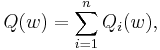
where the parameter  is to be estimated and where typically each summand function
  is associated with the
  -th observation in the data set (used for training).
In classical statistics, sum-minimization problems arise in least squares and in maximum-likelihood estimation (for independent observations). The general class of estimators that arise as minimizers of sums are called M-estimators. However, in statistics, it has been long recognized that requiring even local minimization is too restrictive for some problems of maximum-likelihood estimation, as shown for example by Thomas Ferguson's example.[1] Therefore, contemporary statisticial theorists often consider stationary points of the likelihood function (or zeros of its derivative, the score function, and other estimating equations).
The sum-minimization problem also arises for empirical risk minimization: In this case,  is the value of loss function at -th example, and
  is the empirical risk.
When used to minimize the above function, a standard (or "batch") gradient descent method would perform the following iterations :
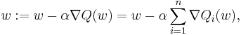
where  is a step size (sometimes called the learning rate in machine learning).
In many cases, the summand functions have a simple form that enables inexpensive evaluations of the sum-function and the sum gradient. For example, in statistics, one-parameter exponential families allow economical function-evaluations and gradient-evaluations.
However, in other cases, evaluating the sum-gradient may require expensive evaluations of the gradients from all summand functions. When the training set is enormous and no simple formulas exist, evaluating the sums of gradients becomes very expensive, because evaluating the gradient requires evaluating all the summand functions' gradients. To economize on the computational cost at every iteration, stochastic gradient descent samples a subset of summand functions at every step.
Iterative method
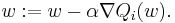
In stochastic (or "on-line") gradient descent, the true gradient of is approximated by a gradient at a single example:
As the algorithm sweeps through the training set, it performs the above update for each training example. Several passes over the training set are made until the algorithm converges. Typical implementations may also randomly shuffle training examples at each pass and use an adaptive learning rate.
In pseudocode, stochastic gradient descent with shuffling of training set at each pass can be presented as follows:
- Choose an initial vector of parameters and learning rate .
- Repeat until an approximate minimum is obtained:
- Randomly shuffle examples in the training set.
- For
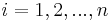 , do:
, do:
There is a compromise between the two forms, which is often called "mini-batches", where the true gradient is approximated by a sum over a small number of training examples.
The convergence of stochastic gradient descent has been analyzed using the theories of convex minimization and of stochastic approximation. Briefly, stochastic gradient methods need not converge to a global minimum unless the objective function is convex --- or more generally unless the problem has convex lower level sets and the function has the monotone property called "pseudoconvexity" in optimization theory, and finally the step-sizes are very small.[2]
Example
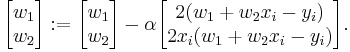
Let's suppose we want to fit a straight line  to a training set of two-dimensional points
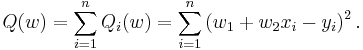
  using least squares. The objective function to be minimized is:
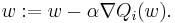
The last line in the above pseudocode for this specific problem will become:
Applications
Some of the most popular stochastic gradient descent algorithms are the least mean squares (LMS) adaptive filter and the backpropagation algorithm.
References
- ^ Ferguson, Thomas S. (1982). "An inconsistent maximum likelihood estimate". J. Am. Stat. Assoc. 77 (380): 831–834. JSTOR 2287314.
- ^ Kiwiel, Krzysztof C. (2001). "Convergence and efficiency of subgradient methods for quasiconvex minimization". Mathematical Programming (Series A) (Berlin, Heidelberg: Springer) 90 (1): pp. 1-25. doi:10.1007/PL00011414. ISSN 0025-5610. MR1819784.
- Bertsekas, Dimitri (2003). Convex Analysis and Optimization. Athena Scientific.
- Bertsekas, Dimitri P. (1999). Nonlinear Programming (Second ed.). Cambridge, MA.: Athena Scientific. ISBN 1-886529-00-0.
- Davidon, W. C. (1976). "New least-square algorithms". Journal of Optimization Theory and Applications 18 (2): pp. 187–197. doi:10.1007/BF00935703. MR418461.
- Stochastic Learning. Lecture by Léon Bottou for the Machine Learning Summer School 2003 in Tübingen. Also in Advanced Lectures on Machine Learning edited by Olivier Bousquet and Ulrike von Luxburg, ISBN 3-540-23122-6, 2004
- Kiwiel, Krzysztof C. (2003). "Convergence of approximate and incremental subgradient methods for convex optimization". SIAM Journal of Optimization 14 (3): pp. 807–840. doi:10.1137/S1052623400376366. MR2085944. (Extensive list of references)
- Pattern Classification by Richard O. Duda, Peter E. Hart, David G. Stork, ISBN 0-471-05669-3, 2000
- Introduction to Stochastic Search and Optimization by James C. Spall, ISBN 0-471-33052-3, 2003
External links
- sgd: an LGPL C++ library which uses stochastic gradient descent to fit SVM and conditional random field models.